Planet Ghibli Part 2 - Making a Video

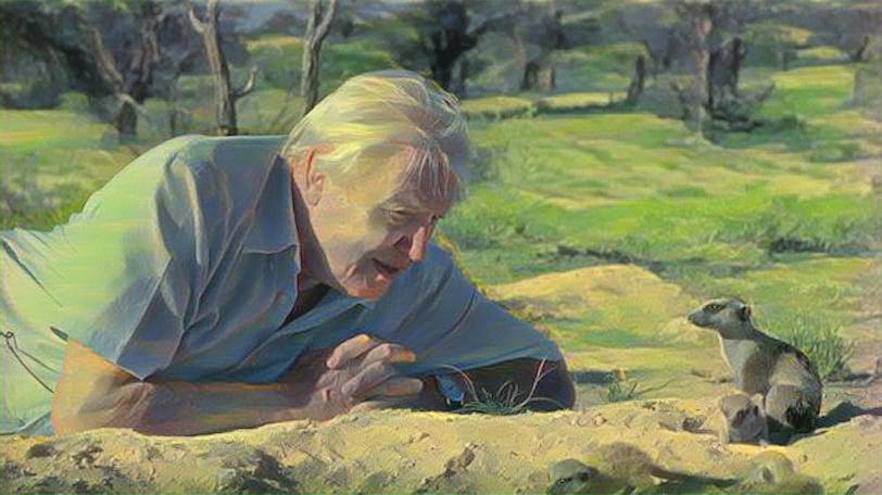
Welcome to the second part of our Planet Ghibli adventure. In the first part, we styled single images and now we shall attempt to style an entire video. The video we will style is this trailer for Planet Earth II.

So how do we do this? Well, the simple and straight forward answer is; we extract all the frames from the video and do the style transfer on each frame.

Quick links for this post (a.k.a. TLDR)

Code repository

Final result: Styled Trailer

Discussion

Before we move on

Remember from Part 1 it took us 1-2 minutes for each image? The trailer is 2 minutes and 46 seconds long, so if we have 24 frames every second… Yeah. That’s almost 4000 images, and thusly around 3 days. For 128 pixel resolution images.

Time to go look for more efficient approaches! One of the fanciest is using something like CycleGAN. But from what I understand looking into it, the computational requirements are high. What might work better is fast neural style transfer (original paper).

This only takes a few seconds per image, if we have a trained model. So what does it mean to have a trained model?

Training models briefly explained

In part 1, our pytorch code used a pre-trained object recognition network to calculate values for images. Someone had already gone through the process of “teaching” this network to recognise objects in images, by “showing” it thousands and thousands of images and pointing out where the objects are¹. By exploiting aspects of this pre-trained object recognition network, we could run our style and input images through it, calculate difference values, and manipulate an output image so that it became a mix between the style and input.

The fast neural transfer also uses a pre-trained object recognition network, but additionally, it trains a “image transformation network” (see Figure 2 in the paper for a nice overview). By running many images through this system, this image transformation network learns to output a styled image without having to calculate any differences between the style, input and output. It just changes the input image into an output image directly.

In other words, we could say that when we train our fast neural transfer, it’s similar to what happens in part 1, but instead of treating each successive image as a new and separate case, the image transformation network will first learn how to style the first image, then it learns how to style the first and second image, then the first, second and third… you get the picture. Hah! Picture. Pun not intended, but pun happened.

The downside here is we need thousands of images to train on. So it will take some time to do this training for our chosen style image, but when it’s done, each frame of our video will only take seconds. So in a way, we’re betting here that the training will take less time than the 3 days or so we estimate to use the method from part 1 to style the entire video.

I should mention that when I make this bet, I take into consideration that I’ve access to a GTX980Ti graphics card at university. It accelerates training significantly compared to my laptop, on which this kind of deep learning is basically pointless. We will discuss this at the end of this post.

Actually training our model(s)

I cloned the git repo mentioned earlier for fast neural style, and used their instructions to train a model using the same style image we used in Part 1. I used the image of Sir David and our custom Planet Ghibli “logo” as test images, as seen here:

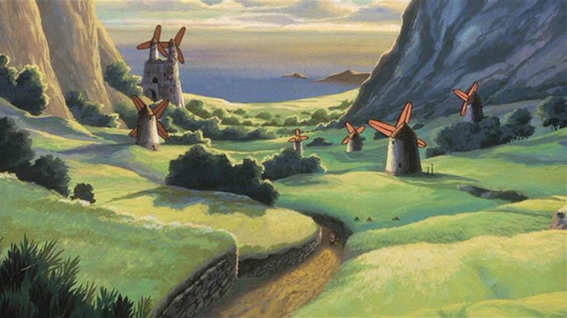
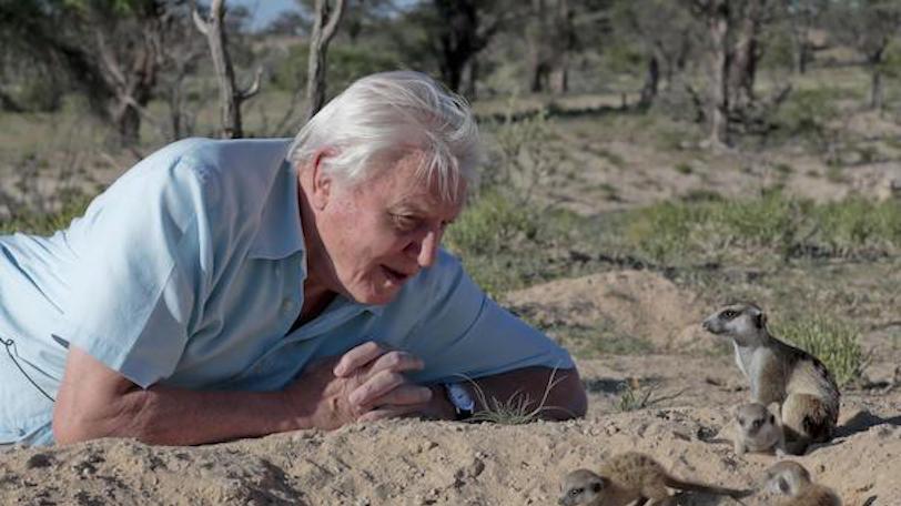
Style image to the far left and our test images to be styled. Click for larger versions.

One training run on the COCO2014 image dataset (the one recommended in their readme), took around 3h using a GTX980Ti for CUDA acceleration. Good thing I’ve access to such a card at the university, or it would likely not have been worth it compared to those 3 days we spoke of in the beginning of this post. Deep learning without GPU acceleration, like on my laptop (and most other non gaming laptops), is basically impossible unless it’s for small toy examples².

The first training run used the default parameter settings for content-weight and style-weight; 1e5 and 1e10, respectively, and gives us these results:

Images styled with style-weight=1e10. Click for larger versions.

These look okay, but to my eyes more like color and blur filters or something than actual style. They don’t look “painting-like” if you get what I mean? Let’s try using style-weight=1e11 instead!

Wait, wait; I hear you. What is this style weight business? Again referring back to Part 1, the style weight tells the training algorithm to give more weight to the style than the content. By adjusting both the style-weight and content-weight parameters we can fine tune the look of our output images. How do we find good values, you ask? Well, my friend, that’s the secret about these things. You have to test and retest. Luckily for us, the readme tells us their example images have used values between 1e10 and 1e11 for the style weight.

So! Another three hours go by and we have a new model to test with our images:

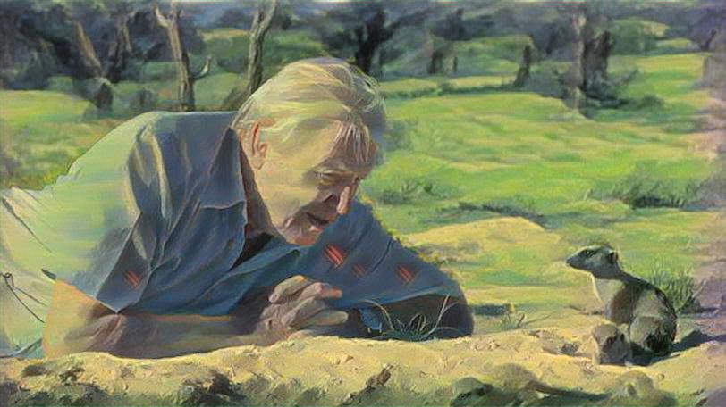
Images styled with style-weight=1e11. Click for larger versions.

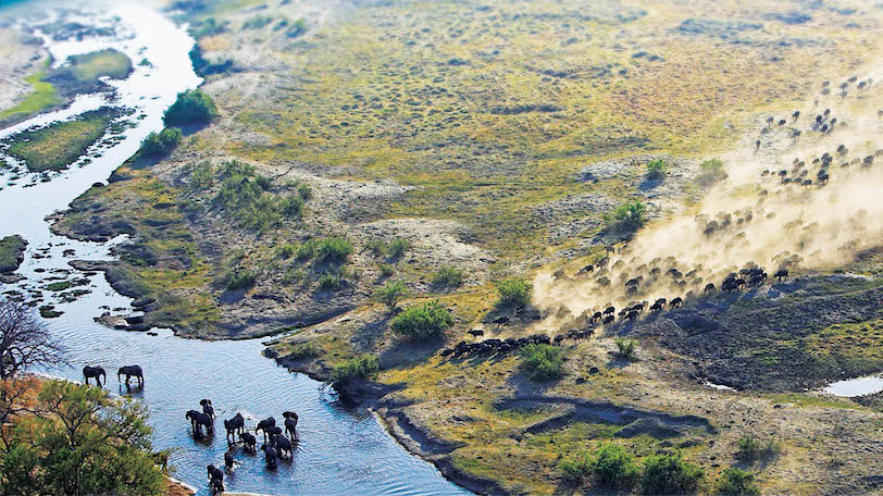
Notice those red stripes on Sir David’s shirt? And in the water in the bottom right of the elephant shot? You recognise it? If not, scroll back up to the style image from Nausicaa that we use. Then continue to the next paragraph.

You’re right, those are the windmill sails! How did they get there? Mayhaps you figured it out already, but remember we just spoke of what style weight does? By increasing the weight - the importance - of the style image over the content images during training, more of the style “seeps through”. In our case, it seems that during training, one of the features identified by the object recognition network, was these sails. Again, looking at the Nausicaa image, those sails do stand out from the rest of the picture so it’s not surprising it’s a stand out feature.

Either way, this isn’t what we want right? Sure, both the test images now look more “painted” but we don’t want those sails. Let’s try using style-weight=5e10, a value in-between the first and second attempts. Another three hours of training and now we get this:

Images styled with style-weight=5e10. Click for larger versions.

These aren’t too bad! To be honest I slightly prefer the results of the method in Part 1, but these are good enough. We have already spent nine hours training, plus a few extra hours fiddling around with the code.

Extracting frames and running the style transfer

I downloaded the trailer using youtube-dl, which if you didn’t know can be used to download video clips from twitter, reddit and other sites as well. Very useful when you want to save those cute animal gifs for future use.

Next step is to use another wonderfully useful little application; ffmpeg³. It can convert between video formats quickly and do many other nifty things with video and audio. For our use case, it can extract all the frames from our trailer into individual jpg files at 24 frames per second:

ffmpeg -i input.mp4 -r 24/1 out%03d.jpg

Then we extract the audio:

ffmpeg -i input.mp4 -q:a 0 -map a audio.mp4

What we get out is almost 4000 images (!), and it’s impressive, at least to me, that this process only takes a few minutes even on my crappy laptop.

Style transfer

Even though the fast style transfer is much quicker than the original one, each image still takes up to 10 seconds on my laptop. That would be 11h for 4000 images. So again, I use the office graphics card, which takes only 12 minutes in total. That’s because our image dataset easily fits into the memory of the graphics card, and pytorch intelligently identifies this and transfers all the images to the graphics memory, converts them, and then sends the images back to the CPU and saves to disk.

Also, the code we’re using has no support to do many images in batch, so I created a wrapper file, which I uploaded to my forked repository on GitHub.

Putting the pieces back together

With all the images styled and downloaded to my laptop, we use ffmpeg to put the pieces back together:

ffmpeg -r 24 -i out%03d.jpg -i audio.mp4 -c:v libx264 -c:a mp3 -r 24 -shortest output.mp4

The above command assumes you have not changed the filenames from the extracted ones :)

The final result can be seen on Vimeo

Discussion

If you check out the vimeo video, you’ll see that some scenes don’t look that great. Others look really cool! So like in the previous post, we see this interaction between input and output where we can’t be sure of how things turn out until we try it.

When we trained our model we used an existing dataset of thousands of images, training our image transformation network to output styled images in a way that’s an average of all those thousands of pictures. So it could be the case we would get better results if we either trained on extracted images from the trailer. Another way to improve the result would be to have separate transformation networks for different parts of the trailer. For example, if there are lots of details in the image, like in an aerial shot of a horde of animals or a forest scene with many leaves and branches; that would be one category or model variant. Another variant could be when there’s a close up shot of an animal. We could also go back to the image used for styling, perhaps another kind of image would work better for some scenes?

Since I don’t have much experience with style transfer, I cannot say what approach would be best or has the highest chance of producing better results. Perhaps it would be a waste of time to try any of the suggestions I gave, because we actually should look at another neural network architecture or maybe we just can’t get noticeably better results.

What (hopefully) does become obvious here is that machine learning involves lots of trial and error. As mentioned above, it took three hours to train the style model on a 980Ti GPU. Its launch price in 2015 was $649, but can still be found on ebay for £100-200. This graphics card needs 250w, excluding the energy needs of the rest of the system. So there’s a decent amount of energy use here, especially adding that we had to train for 3x3h to find a good parameter setting.

There are analyses of compute cost (open ai) and/or energy and cash cost (yuzeh) of machine learning, but they only take the final training cost into consideration. What I mean is, if they would talk about my simple experiment here they would use the 3h number to calculate compute, energy and money cost⁴. Even if they take all self-play matches of AlphaZero into consideration, they don’t consider all the testing it took to find the parameter values they would use for all those self-play matches!

But wait, there’s more! We have only mentioned the trial and error procedure to find the right parameters when we have the right architecture.

What about coming up with the architecture in the first place? It’s not easy, and is a combination of experience and exploration. I honestly don’t know how much you can predict mathematically about the performance and output effects of different architectures, as that’s not my research area. I do know that it’s a very active field of research though, because we simply don’t know enough about how neural networks function, leading to for example the “lottery ticket hypothesis” about using bigger neural networks. In short, it means there’s trial and error in finding a good architecture as well.

It’s uncommon these efforts are mentioned in papers presenting results, or even in discussions such as those referenced above about compute cost, which is unfortunate. It can give the impression that machine learning, especially using neural networks, is easier than it actually is. The resource costs to get into this kind of research are enormous, and even if you had lots of money, you would need expertise and experience to not waste those resources.

If we look at deep reinforcement learning research (deep RL) for example, this becomes even more apparent. In deep RL research, the most common task is to get machine learning systems to play video games. In a rare example of transparency (though still glossed over), the paper presenting pysc2 - a python framework to play Starcraft 2 - has a few graphs like this:

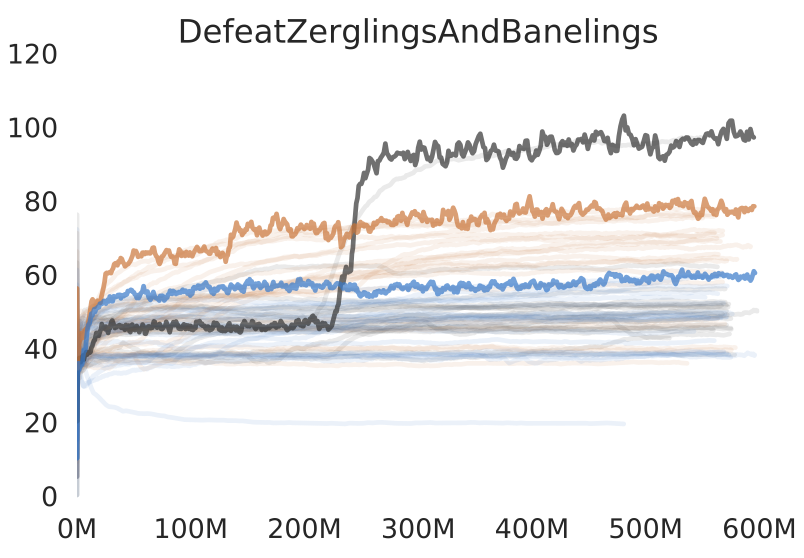
Graph from pys2c paper showing score on the vertical axis and time steps on horisontal axis. The different colours represent different architectures for the neural net.

It doesn’t really matter what the task is that this graph represents, it could be any task. Each colour is a different neural network architecture, and the bold lines are the best results for each architecture. The faint lines are what I want to point out. These faint lines grey lines are using the same architecture as the winning thick grey line, but uses different hyperparameters. Meaning, parameters such as the style weight and content weight we had to trial and error for the style transfers.

So, not only did they run 100 experiments for each architecture. If we read this graph right, it looks like only two of those 100 experiments for the winning grey architecture rose high above the others. And you would not even know that until after around 200 million time steps. Additionally, if we look at averages across all the lines of each colour, doesn’t it look like the orange architecture is better overall? If so, the researchers have actually chosen outliers as their presented result!⁵

Are you starting to grasp the enormous amount of work put into something that works?

It’s no wonder Deepmind and OpenAI have hundreds of top-of-the-line PhD graduates for research and millions of dollars in backing to fund the computational resources they require. Looking at recent advances in text generation, specifically GPT-3, it’s an enormous computational achievement that’s only feasible for large and well funded organisations.

Conclusions and up next

To conclude, machine learning and deep learning in particular are expensive activities. One could question if it’s worth the climate costs. And what are the societal costs and effects when only huge companies can train these systems?

In the next post we shall touch on those questions. We will also discuss the input/output relationship we have seen both here and in part 1; how we need to test and evaluate output depending on the input. If we are not careful, we can cause real issues in society so it’s important to discuss the implications of magic input-output boxes.

Edit: Now available at a server near you: Part 3